Dijkstra's Algorithm

What is a Weighted Graph?

A weighted graph is a graph where each edge has a weight or cost associated with it. This weight can represent distances, time, or any cost metric depending on the problem domain.

---

Dijkstra’s Algorithm

Breadth-First Search (BFS) finds the path with the fewest segments, but it does not consider weights that’s where Dijkstra Algo is used.

Steps of Dijkstra’s Algorithm:

1. Find the cheapest node (i.e., the node with the lowest cost from the starting node).
2. Update the cost of its neighbors if a cheaper path is found.
3. Mark the node as processed and repeat until all nodes have been processed.
4. Calculate the final shortest path by backtracking the parent nodes.

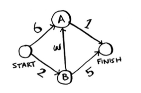
Example 1

Node	Cost	Parent
Start	0	-
A	6	Start
B	2	Start
Fin	Inf.	-

Step 1: B is the cheapest node from start

Step 2: Update cost of B’s neighbours

• A(cost = 2+3=5) and since 5<6, update A’s cost and change parent to B.
• Fin. (cost=2+5=7) and since 7<Inf., update Fin. cost and change parent to B.

Node	Cost	Parent
Start	0	-
A	5	B
B	2	Start
Fin	7	B

Step 1(Second Time): Cheapest node is A

Step 2(Second Time): Update cost of A’s neighbours

• Fin. (cost=5+1=6) and since 6<7, update Fin’s cost and change parent to A

Node	Cost	Parent
Start	0	-
A	5	B
B	2	Start
Fin	6	A

Since FINISH has no outgoing edges, Dijkstra’s Algorithm is complete. Finish → Parent is A → Parent is B → Parent is Start.

Final Shortest Path: Start → B → A → Finish

---

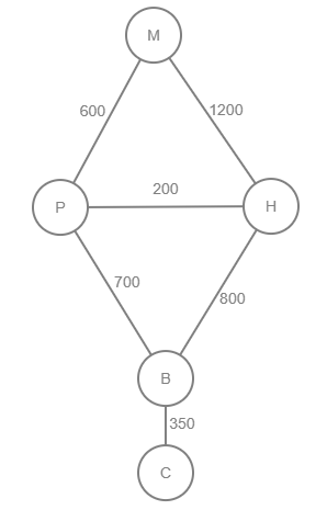
Example 2

City	Cost	Parent
Mumbai	0	-
Pune	600	Mumbai
Hyderabad	1200	Mumbai
Bangalore	∞	-
Chennai	∞	-

Step 1: Pune is cheapest

Step 2: Update neighbours of Pune

• Bangalore (600 + 700 = 1300 km)
• Hyderabad (600 + 200 = 800 km, updated from 1200 km)

City	Distance from Mumbai	Parent
Mumbai	0	-
Pune	600	Mumbai
Hyderabad	800	Pune
Bangalore	1300	Pune
Chennai	∞	-

Step 1(Second Time): Hyderabad is cheapest

Step 2(Second Time): Update neighbours of Hyderabad

• Pune(800 + 200 = 1000 km ), Discarded as 1000km >600Km
• Bangalore (800 + 800 = 1600 km, Discarded as 1600Km>1300km

City	Distance from Mumbai	Parent
Mumbai	0	-
Pune	600	Mumbai
Hyderabad	800	Pune
Bangalore	1300	Pune
Chennai	∞	-

Step 1(ThirdTime): Bangalore is cheapest

Step 2(Third Time): Update neighbours of Bangalore

• Chennai(1300 + 350 = 1650 km )

City	Distance from Mumbai	Parent
Mumbai	0	-
Pune	600	Mumbai
Hyderabad	800	Pune
Bangalore	1300	Pune
Chennai	1650	Bangalore

Since Chennai is last city, no new updates

Final shortest path : Mumbai → Pune → Bangalore → Chennai ( Total dist = 1650km)

---

Dijkstra’s Implementation

function Dijkstra(graph, start):
    costs = {}  # Stores shortest known distance to each node
    parents = {}  # Stores the previous node for shortest path tracking
    processed = []  # List to track processed nodes

    # Initialize costs and parents
    for each node in graph:
        costs[node] = infinity  # Initially, all nodes are unreachable
        parents[node] = None  # No known parent yet
    costs[start] = zero  # Distance to start node is zero

    # Process the graph
    node = find_lowest_cost_node(costs, processed)
    while node is not None:
        cost = costs[node]  # Get the current node's cost
        neighbors = graph[node]  # Get all neighbors of this node

        for each neighbor in neighbors:
            new_cost = cost + neighbors[neighbor]  # Calculate new cost
            if new_cost < costs[neighbor]:  # If new path is shorter, update
                costs[neighbor] = new_cost
                parents[neighbor] = node

        processed.append(node)  # Mark the node as processed
        node = find_lowest_cost_node(costs, processed)  # Get next node

    return costs, parents  # Shortest paths from start node

Running Time - The algorithm processes each node once and updates neighbors, making its time complexity:

• O(V²) using a simple array
• O((V + E) log V) using a priority queue (Heap)